2nd order analysis
Theory
The second-order analysis is a powerful tool for engineers when designing slender frame structures. Views on the scope of its use, however, differs along the engineering community. Therefore, this chapter clarifies some important aspects of this theory both from practical and theoretical point of view.
The theory of second-order is a tool for stress analysis of slender structures with significant axial forces that are either under the effect of lateral forces, or are exposed to initial imperfections. Imperfections can be material ones (eg. Uneven distribution of stiffness in the cross-section) or geometric ones (curved member axis eccentricities in supports etc.). Material imperfections can be usually converted into geometric ones. In this case, the member axis in imperfect structures means a line connecting stiffness centres of heterogeneous sections.
The second order theory is a simplification method of geometrically non-linear analysis of structures. The assumptions upon which this theory can be used, are listed below. The difference between the geometrically non-linear and linear approach can be shown in the following figure:
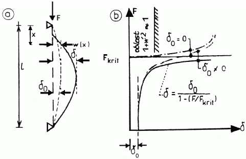 Loading curves of ideal (δ0=0) and imperfect (δ0≠0) member
In the first part of the figure, the initial imperfections are expressed by the parameter δ0 and the final state by the parameter δ. The initial imperfections δ0 may be caused also by the effect of lateral forces. They can be determined by the common calculation according to the first order theory. Second part shows the loading curves of ideal (δ0=0) and imperfect (δ0≠0) member corresponding to the geometrically non-linear (dashed curves) and linear (solid curve) solutions. They can be obtained by integrating the differential Euler equation:
![]()
For the geometrically non-linear analysis following expression can be used:

This expression is valid for linear analysis:
![]()
Apostrophe means the derivation of deflection. As the integrating of the Euler differential equation is difficult, the approximate methods are usually used. Here, the deformation variant of FEM is used.
Geometrically non-linear calculations are necessary to find critical states (bifurcation or limit ones) on the diagram "load-displacement" especially for curved structures, such as arches and meshed structures arranged in the shape of a curved surface (e.g. spherical or cylindrical). In a limit point, load reaches its maximum or minimum value. The bifurcation points leads to branching of balance (e.g. intersection of symmetrically and non-symmetrically deformed arch). As the linear calculation (dotted line) is not able to cover these relationships, it significantly overestimates the stability capacity.
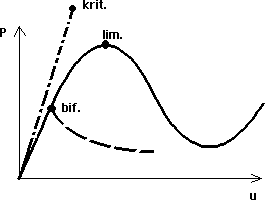 Bifurcation and limit points
Linear calculations can be applied with certainty to the common frame structures forming an orthogonal system (option a in the following figure). Contrary to structure a, the structure b acts closer to the arch c and the linearisation is inadmissible. The decision whether the design can use linear or non-linear calculation requires not only the theoretical knowledge but also some practical experiences.
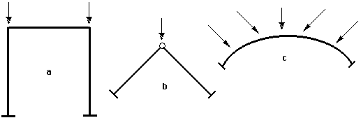 Validity of linear theory
Assumptions of second order theory
The second order theory is a simplification of non-linear analysis and is based on following assumptions:
- The relation between deformations and movements are linear
- The internal forces don't change during deformation
- Equilibrium is calculated on deformated structure
With the classical formulation based on the integration of basic equations, the relationship between end member forces f and corresponding movements r can be expressed using formula
![]()
Where is: | λ |
|
All external forces grow proportionally to this parameter. Linearity of the analysis means that the stiffness matrix K is not a function of the joint deformations vector r. There are two ways how to solve the problem.
First way is, that the stiffness matrix K(λ) is converted using expression
![]()
Where is: | K0 |
|
Kσ |
|
The solution is close to the exact results, if the member division is satisfactory. This approach is the basis of programs. In accordance with the above formulation, the following calculation is used. The first step is to determine the axial forces on the structure using the first order theory. Knowledge of the axial forces is used for composition of initial stress matrix Kσ. The calculation is repeated after that, however, with modified matrix K(λ).
The basic equation assumes ideal shape of structure, but with the possibility of lateral load forces. In the case of imperfect structure loaded with axial forces, the expression is modified accordingly:
![]()
Where is: | r0 |
|
The expression K0r0 is equal to the effect of shear forces. In case of combination of both effects, the impacts of imperfections K0r0 and shear forces R are added up. If both expressions K0r0 and R are equal to 0, the analysis turns into the problem of linear stability.
Second solution is based on the classic principles of analysis of slender imperfect structures.
The fundamental equation is
![]()
The stiffness matrix is updated with the respect of new geometry, therefore
![]()
The inbalance f≠K1r can be developed by this expression
![]()
or
![]()
The calculation is repeated until
![]()
Second order theory and standards
Designing standards are based on the determination of buckling coefficients, that correspond to the member slenderness (buckling lengths). Used expressions are based on the fundamental assumption that the member is isolated. However, members are usually part of a structure and are affected by surrounding members. Therefore, buckling lengths are usually different. As the second order theory provides internal forces on deformed structure, there is no need to calculate buckling coefficients. It can be said that the stability problem is thus converted into the strength analysis.
Finally, one important conclusion. Knowing the value of the critical load factor λcrit, we can easily estimate the deformation according to the second order theory with respect to initial imperfections δ0 or deformations calculated according to the first order theory (providing that the load is proportional and the decisive members are compressed).
![]()
Similar expressions may be used (with lower precision) also for internal forces like bending moments etc.
![]()
Where is: | M0 |
|
Example
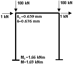
Short example shows the validity of the relationships mentioned above. The example is a simple plane frame loaded by point loads in the corners of the frame. The geometric imperfections were simulated by lateral forces with the magnitude 1/100 of the vertical force. Horizontal movement of beam δ0 calculated according to the first order theory is equal to 0.659mm. Second order analysis calculates the horizontal displacement δ equal to 0.675mm. Similar results were obtained for the bending moment in supports. Moment M0 was equal to 1.66kNm, while moment M calculated according to the theory of second-order rose to 1,69kNm. Using the equations above, the lateral displacement δ is equal to 0.676 mm, which practically coincides with the calculation using the FIN 3D. The value of the bending moment is equal 1,70kNm. The difference is less than 0.6%.
 Structure scheme